CVXOPT HW2
$\newcommand{R}{\mathbb{R}}$
1) Consider the optimization problem
$$\min f_0(x_1, x_2)$$ Subject to $$2x_1 + x_2 \ge 1$$ $$x_1 + 3x_2 \ge 1$$ $$x_1 \ge 0, x_2 \ge 0$$
Make a sketch of the feasible set. For each of the following objective functions, give the optimal set and the optimal value
a) $f_0(x_1, x_2) = x_1 + x_2$
$f_0$ is an affine function. The constraints are all affine. Even without any formal properties, we can see that the solution is most likely to be in the “vertices”. Our vertices here are $(0, 1), (1, 0), (0.4, 0.2)$. Let us evaluate the function at each of these points
- $f(0, 1) = 1$
- $f(0.4, 0.2) = 0.6$
- $f(1, 0) = 1$
Out of the vertices, $(0.4, 0.2)$ is the minimum. We know that since $f_0$ is strictly increasing, it order to minimize we need to move in the negative direction along both axes. But we cannot possible move in that direction as $(0.4, 0.2)$ is our boundary. Hence we have to settle for a bit of positive direction in either one of the axes.
Just as a sanity check let us evaluate function on the neighbours.
Let us move along the negative direction along $x_1$. Setting $x_1 = 0.39$ we get $x_2 = 1-2x_1 = .22$ and our $f_0$ is $0.61$.
Similarly if we move along the negative direction along $x_2$. Setting $x_2 = 0.19$ we get $x_1 = 1-3x_2 = 0.43$ and $f_0 = 0.62$.
Hence the optimal set is $\boxed{(0.4, 0.2)}$ and the optimal value is $\boxed{0.6}$
b) $f_0(x_1, x_2)= -x_1-x_2$
Notice that we can write this as $-(x_1 + x_2)$. This is strictly decreasing and our constraints allow us to move towards $+\infty$. It is unbounded in that direction. We don’t have a solution here.
c) $f_0(x_1, x_2) = x_1$
This is just minimizing $x_1$.
The optimal set is $\boxed{(0, x_2), x_2\ge1}$ and the optimal value is $0$. This just gives the y-axis > 1.
d) $f_0(x_1, x_2) = \max{x_1, x_2}$
The function gives the larger coordinate out of the two. This corresponds to the $y=x$ line splitting $\mathbb{R}^2$ into two. In order to minimize this function, we need to find the smallest $x_1$ greater than the smallest $x_2$ or vice-versa.
We can write that as $\min_{x\in x_1} {x \ge \min x_2}$ or $\min_{x\in x_2} {x \ge \min x_1}$ Geometrically we’re trying to move down from $(0, 1)$ along $2x_1+x_2\ge 1$ and we’re trying to move up from $(1, 0)$ along $x_1+3x_2 \ge 1$ We see that the minimizer is ${\frac{1}{3}, \frac{1}{3}}$ Moving up or down give a value greater than $\frac{1}{3}$
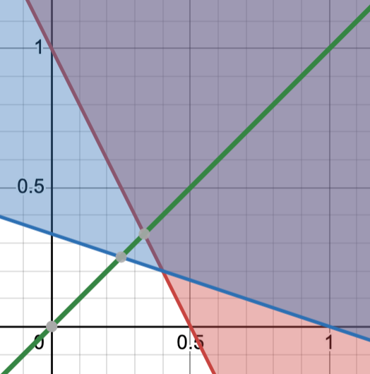
$e) f(x_1, x_2) = x_1^2 + 9x_2^2$
We see that this is a paraboloid centered at $(0, 0)$. We are only concerned with the positive quadrant, hence we get a pie shape. Since this is convex, we know that the optimal points lie near the vertices. Since we have the equations of the lines, we can parameterize $x_2$ and convert this into a univariate problem. Then we just have to analyze the values of $f_0$ along this $\mathbb{R}^1$ strip. We split this into two regions - $[0, 0.4], [0.4, 1]$.
Let us first consider $[0, 0.4]$, in this region $x_2 = 1 - 2x_1$, then our objective function becomes $x_1^2 + 9(1 - 2x_1)^2 = 37x^2 - 36x + 9$
Differentiating, we get
$$f’(x) = 74x - 36$$
Setting to 0, we find the minima at
$$x = \frac{36}{74} = .48648648648648648648$$
Which is not in the domain.
We see that $f’(x) < 0, x\in[0, 0.4]$, hence the local minima is at $0.4$
The value at $f_0(0.4, 0.2) = 0.52$
In the other domain
Here $x_2 = \frac{1 - x_1}{3}$ $$f_0(x)= x^2 + 9\left(\frac{1 - x_1}{3}\right)^2$$ $$f_0(x)= x^2 + 9\left(\frac{1 + x^2 - 2x}{9}\right)$$ $$f_0(x)= x^2 + 1 + x^2 - 2x$$ $$f_0(x)= x^2 + 1 + x^2 - 2x$$ $$f_0(x)= 2x^2 -2x + 1$$ Differentiating $$f’(x) = 4x - 2$$ The minima is at $x = 0.5$ which is in the domain The value is then $f_0(1/2, 1/6) = 0.5$
Hence the optimal set is $\boxed{(1/2, 1/6)}$ and the optimal value is $\boxed{0.5}$
2) Linear Programming
Consider you need to ship $n$ products from $m$ warehouses to $n$ destinations. Each warehouse can ship to at most one product to a single destination (we can assume $m \ge n$). The distance from the $i^{th}$ warehouse to the $j^{th}$ destination is given as $d_{ij}$. You want to ship all the $n$ products with minimal total distance travelled. Set this problem up as a linear programming problem, with $x_{ij} = 1$ if the $i^{th}$ factory ships to the $j^{th}$ destination, and $x_{ij} = 0$ otherwise. However, to make this a linear programming problem, rather than discreate optimization, set up the optimization variables $x_{ij}$ to be continuous and constrained within $[0, 1]$
a) Write down a formula for the objective function $f(x)$ and the inequality/ equality constraint functions. This should be in the standard form of a linear programming problem.
Before converting this to the standard form, let us worry about just expressing these constraints as a Linear optimization problem.
Let us remind ourselves what a linear optimization problem looks like (not necessarily in standard form)
$$\min c^T x + d$$ subject to $$Gx \preceq h$$ $$Ax = b$$ Where $x\in R^n, G\in\R^{m\times n}, h\in\R^m, A\in\R^{p\times n},b\in\R^p$
As suggested in the question, we can express $X$ as a $\R^{mn}$ column vector $x$ rather than $\R^{m\times n}$ matrix.
Similary, we can express the distance matrix $D$ as a column vector $c$
As we don’t have any $d$, our objective function becomes $c^Tx$
Next we have to worry about the constraints. They are, in natural language, as follows:
- Each warehouse ships to atmost one destination
- All destinations have atleast one warehouse shipping to them i.e no destination is left out.
- The values of $x$ are in $[0, 1]$
Though they seem very simple written in English, we have to express these using matrix multiplication, which may be hard. The third constraint, converting the discrete problem to a continuous one, makes this harder. We have to ensure that this domain expansion doesn’t affect the first two constraints.
How do we interpret this domain expansion? Can we interpret it as a probability distribution since the values are restricted to $[0, 1]$? Or can we think of it as a weighted average? Either way, we see that we can translate the constraints as follows:
- $x_{ij} \ge 0 \implies x \succeq \mathbf{0} \implies -x \preceq \mathbf{0}$
- $\sum_{i\in[m]} x_{ij} = 1$
- If we think of each $x_{ij}$ as the probability that warehouse $i$ ships to destination $j$, then the probability that destination $j$ gets anyone to ship to it should be 1. Combining with the above inequality, this leads to $x_{ij} \le 1, \forall i,j \implies x \preceq \mathbf{1}$
- $\sum_{j\in[n]}x_{ij} \le 1$
- Again through the lens of probability, this constraint ensures that the probability that warehouse $i$ ships at all is a valid one. This has the effect of making sure that a warehouse $i$ can only deliver to atmost one destination with absolute certainty (This is very hand wavy, but the constraint does make sure that a warehouse only ships to one destination)
With these constraints, we now have valid probability distributions both row-wise and column-wise on our matrix $X$. Constraining to become a valid probability distribution also satisfies the constraints of our problem.
Let us represent them in terms of matrices. Looking at inequality constraints first,
$$-x \preceq \mathbf{0}$$ $$-I_{mn}x \preceq \mathbf{0}$$ $$ \begin{bmatrix} -1 & 0 & \ldots & 0 \ 0 & -1 & \ldots & 0 \ \vdots & \vdots & \ddots & \vdots \ 0 & 0 & \ldots & -1 \ \end{bmatrix} \begin{bmatrix} x_{11}\ \vdots\ x_{1n}\ \vdots\ x_{m1}\ \vdots\ x_{mn}\ \end{bmatrix} \preceq \begin{bmatrix} 0 \ \vdots \ 0 \end{bmatrix} $$
To express $\sum_{j\in[n]}x_{ij} \le 1$ we essentially need to dot every row of $X$ with $\mathbf{1}$. Abusing notation, we can express this as
$$ \begin{bmatrix} \mathbf{1}^T & 0 & \ldots & 0\ 0 & \mathbf{1}^T & \ldots & 0\ \vdots & 0 & \ddots & \vdots\ 0 & 0 & \ldots & \mathbf{1}^T \end{bmatrix} \begin{bmatrix} x_{11}\ \vdots\ x_{1n}\ \vdots\ x_{m1}\ \vdots\ x_{mn}\ \end{bmatrix} \preceq 1 $$
Here $\mathbf{1}\in\R^n$
For $\sum_{i\in[m]} x_{ij} = 1$ we need to select all the $x_{ij}$ for some $j$ Let us introduce some notation to make our lives easier. The vector $\mathbf{e}_x$ corresponds to the basis vector of the $x^{th}$ coordinate. For example, $\mathbf{e}_1$ corresponds to $(1, 0, 0, \ldots)$. to select every $j^{th}$ coordinate, we just multiply $m$-$\mathbf{e}_j$s with $x$. Using this we can express our equality as $$ \begin{bmatrix} \mathbf{e}_1^T & \ldots & \mathbf{e}_1^T\ \mathbf{e}2^T & \ldots & \mathbf{e}2^T\ \vdots & \vdots & \vdots \ \mathbf{e}n^T & \ldots & \mathbf{e}n^T\ \end{bmatrix} \begin{bmatrix} x{11}\ \vdots\ x{1n}\ \vdots\ x{m1}\ \vdots\ x{mn}\ \end{bmatrix}
\mathbf{1} $$
Each $\mathbf{e}\in\R^n$, so each row has $m$ $\mathbf{e}$s, making its dimension $mn$.
Hence, we can state the problem as:
$$\min c^Tx$$ subject to $$ \begin{bmatrix} \mathbf{1_{n}}^T & 0 & \ldots & 0 \ 0 & \mathbf{1_{n}}^T & \ldots & 0 \ \vdots & 0 & \ddots & 0 \ 0 & 0 & \ldots & \mathbf{1_{n}}^T \ &&-\mathbf{diag}(\mathbf{1}{mn})\ \end{bmatrix} x \preceq \begin{bmatrix} \mathbf{1}{m} \ \mathbf{0}_{mn} \end{bmatrix} $$ $$ \begin{bmatrix} \mathbf{e}_1^T & \ldots & \mathbf{e}_1^T\ \mathbf{e}_2^T & \ldots & \mathbf{e}_2^T\ \vdots & \vdots & \vdots \ \mathbf{e}_n^T & \ldots & \mathbf{e}_n^T\ \end{bmatrix} x = \mathbf{1}_n $$
Let us convert this to the standard form $$\min c^Tx$$ $$Gx + s = h$$ $$Ax = b$$ $$x\succeq 0$$
Where $s$ is a slack variable intended to convert the inequality to an equality. In our case, $s$ would be $$ \begin{bmatrix} 1 - G_{\text{upper}}x\ x \end{bmatrix} $$ Here we use $G_{\text{upper}}$ to represent the first $m$ rows of $G$. This essentially is probability that some warehouse $i$ doesn’t ship at all. We see that this $s\succeq 0$
Since $x\succeq0$ is part of the standard form itself, we can remove that. Hence we just have,
$$ \begin{bmatrix} G_{\text{upper}} && I \end{bmatrix} \begin{bmatrix} x \ s \end{bmatrix} = \mathbf{1} $$
We also had the equality constraint with the $\mathbf{e}$ vectors Adding that in, we get $$ \begin{bmatrix} \begin{matrix} \mathbf{1}^T & 0 & \ldots & 0\ 0 & \mathbf{1}^T & \ldots & 0\ \vdots & 0 & \ddots & \vdots\ 0 & 0 & \ldots & \mathbf{1}^T \end{matrix} && I_{m\times m} \ \begin{matrix} \mathbf{e}_1^T & \ldots & \mathbf{e}_1^T\ \mathbf{e}_2^T & \ldots & \mathbf{e}_2^T\ \vdots & \vdots & \vdots \ \mathbf{e}_n^T & \ldots & \mathbf{e}n^T\ \end{matrix} && 0{n\times m} \ \end{bmatrix} \begin{bmatrix} x \ s \end{bmatrix}
\mathbf{1} $$
Concretely, let us see an example for $m = n = 2$ $$ \begin{bmatrix} 1 & 1 & 0 & 0 & 1 & 0 \ 0 & 0 & 1 & 1 & 0 & 1 \ 1 & 0 & 1 & 0 & 0 & 0 \ 0 & 1 & 0 & 1 & 0 & 0 \ \end{bmatrix} \begin{bmatrix} x_{11} \ x_{12} \ x_{21} \ x_{22} \ s_{1} \ s_{2} \end{bmatrix}
\mathbf{1} $$
b) Assuming all of the distances are strictly positive, i.e, $d_{ij} > 0$, give an argument for why the optimal solution will actually always be at integers, i.e., each $x_ij^* = 0\text{ or }1$
The smallest possible proof of this is that our original matrix $A$ is totally unimodular and any LP program with a unimodular inequality matrix has integral optimal solutions.
But a much simpler and more intuitive argument can be made geometrically.
We already know that, for any convex optimization problem, if the gradient of the objective function is not zero inside the feasible region, then the optimal point lies on the boundary.
As LP is a type of convex optimization problem, it applies here too. But our case is making the distinction between the edge and the vertex.
We already have a theorem stating that there exists an optimal point on the vertex for a linear program. But this theorem is not an if and only if. If we are unfortunate an entire edge, which includes a vertex, can be the optimal set. Our task is to prove that this never happens in this problem.
Let us visualize what this unfortunate scenario really means. An edge represents an equality constraint i.e moving along that edge keeps something constant. If an entire edge is the optimal set that means that the objective function remains constant along this edge.
Let us remind ourselves what our objective function is. $$c^Tx = \sum_i c_i x_i$$ The distances are strictly positive i.e. $c_i >0, \forall i$
For simplicity let us just have 2 warehouses and 2 destinations
Our objective value is $x_1d_1 + x_2d_2$ Let’s suppose that $d_1 \lt d_2$, for any point on the edge that is not the vertex, you can always take some of $x_2$ and give to $x_1$ to make the whole sum smaller. This is the same argument we made for why an interior point can’t be the minima. Hence, this movement will continue till we reach $x_1 = 1, x_2=0$.
For strictly positive unique distances, the solution is always on the vertices. This points a greediness nature. Though, I cannot formally reduce it, this look very similar to the 0-1 knapsack problem.
CEX
For 2 warehouses and 2 destinations,
$d_{ij} = \begin{bmatrix}1 \ 1 \ 1\ 1\end{bmatrix}$
Both $x = \begin{bmatrix}0.5 \ 0.5 \ 0.5 \ 0.5\end{bmatrix}$ as well as $x = \begin{bmatrix}1 \ 0 \ 0\ 1\end{bmatrix}$ are optimal solutions.
This is a valid instance of the problem. $d_ij > 0$ and the probabilities sum up to 1 both row and column-wise.
I believe distances are unique should be added to the constraints to result in integral solutions as you can establish an ordering amongst them.
d) Modify the problem for the case that each factory can ship an unlimited number of products. What are the new constraint functions? Give an analytic solution to this problem.
We remove the summation condition on the rows. Only the summation condition on the columns and $x$ being in the non-negative orthant remains. The new problem looks like
$$\text{minimize } c^Tx$$ subject to $$Gx \preceq h$$ $$Ax = b$$
Substituting our conditions $$\text{minimize } c^Tx$$ subject to $$x \preceq 1$$ $$-x \preceq 0$$ $$ \begin{bmatrix} \mathbf{e}_1^T & \ldots & \mathbf{e}_1^T\ \mathbf{e}_2^T & \ldots & \mathbf{e}_2^T\ \vdots & \vdots & \vdots \ \mathbf{e}_n^T & \ldots & \mathbf{e}_n^T\ \end{bmatrix} = \mathbf{1} $$
Analytical Solution
If we remove the restriction on the number of destinations that can be served by a warehouse, then the minimization problem is merely picking the closest warehouse from each destination and setting it’s $x$ to be 1.
For the problem above
$$ \begin{matrix} & \text{Destinations}\rightarrow\ \text{Warehouses}\downarrow & \begin{bmatrix} 150 & 37 & 88 \ 23 & 42 & 16 \ 105 & 34 & 7 \ 200 & 95 & 12 \end{bmatrix} \end{matrix} $$
We have 4 warehouses and 3 destinations
The solution for this would be $$ \begin{bmatrix} 0 & 0 & 0 \ 1 & 0 & 0 \ 0 & 1 & 1 \ 0 & 0 & 0 \end{bmatrix} $$
Warehouse 3 serves both destination 2 and destination 3
3) Prove that $x^* = (1, 1/2, -1)$ is optimal for the optimization problem
$$\text{minimize} (1/2)x^TPx + q^Tx + r$$ $$\text{subject to }-1 \le x_i \le 1, i=1, 2, 3,$$
Where $$ P = \begin{bmatrix} 13 & 12 & - 2 \ 12 & 17 & 6 \ -2 & 6 & 12 \end{bmatrix}, q = \begin{bmatrix} -22.0 \ -14.5 \ 13.0 \end{bmatrix}, r = 1 $$
Immediately we notice the quadratic form. But we have to make sure that $P\in S^n_+$. We see that it is symmetric and we verify that it is Positive semi-definite below.
We know that optimality criteria for a differentiable convex optimization problem is
$$\nabla f_0 (x)^T(y - x) \ge 0, \forall y \in \mathbf{dom} f_0$$
Let us calculate the gradient
$$\nabla_x f_0 = \nabla_x\left( (1/2)x^TPx + q^Tx + r \right)$$ $$\nabla_x f_0 = Px + q$$
Evaluating this at $x^* = (1, 1/2, -1)$ we get
$$ \begin{bmatrix} 13 & 12 & - 2 \ 12 & 17 & 6 \ -2 & 6 & 12 \end{bmatrix} \begin{bmatrix} 1 \ 1/2 \ -1 \end{bmatrix} + \begin{bmatrix} -22.0 \ -14.5 \ 13.0 \end{bmatrix} $$ $$
\begin{bmatrix} 21 \ 14.5 \ -11 \end{bmatrix} + \begin{bmatrix} -22.0 \ -14.5 \ 13.0 \end{bmatrix} $$ $$
\begin{bmatrix} -1\ 0 \ 2 \end{bmatrix} $$ Substituting this in the optimality criterion, we get $$ \begin{bmatrix} -1&0&2 \end{bmatrix} \begin{bmatrix} y_1 - 1 \ y_2 - 0.5 \ y_3 + 1 \end{bmatrix} \ge 0 $$ $$ = y_1 + 1 + 2y_3 +2\ge 0\ = y_1 +2y_3 +3 \ge 0 $$
Our domain is $[-1, 1]$ for all our $y$s
It’s clear that this is always greater than 0 if $y_1, y_2 \ge0$
What happens in the negative case?
Substituting the smallest $y$s we get
$$ -1 + 2(-1) + 3 \ge 0\ -3 + 3 \ge 0\ 0 \ge 0\ $$
$y_1 = 1$ and $y_2 = -1$ $$ 1 + 2(-1) + 3 \ge 0\ 2 \ge 0\ $$
$y_1 = -1$ and $y_2 = 1$ $$ -1 + 2(1) + 3 \ge 0\ 4 \ge 0\ $$
Hence this term is always greater than 0 which implies that our $x^*$ is indeed optimal.
4) Suppose $\mathcal{G} = {Q_1, \ldots, Q_k} \subseteq \R^{n\times n}$ is a group, i.e, closed under products and inverse. We say that the function $f: \R^n \rightarrow \R$ is $\mathcal{G}$-invariant, or symmetric with respect to $G$, if $f(Q_ix) = f(x)$ holds for all $x$ and $i=1,\ldots,k$. We define $\bar{x} = \frac{1}{k}\sum_{i=1}^k Q_ix$, which is the average of x over its $\mathcal{G}$-orbit. We define the fixed subspace of $\mathcal{G}$ as
$$ \mathcal{F} = { x | Q_ix = x, i=1,\ldots,k} $$
a) Show that for any $x\in \R^n$, we have $\bar{x} \in \mathcal{F}$
To belong to $F$, every element of the group $\mathcal{G}$ has to be a multiplicative identity.
We know that $\bar{x} = \frac{1}{k}\sum_{i=1}^k Q_ix$, when this is multiplied by some group element $Q_j$ we get $$ \sum_{i=1}^k Q_j Q_i x $$
Notice that we are multiplying $Q_j$ with every member of the group. The result of this operation is the group itself. This is because a group is the generator of itself. Hence any $\bar{x}$ remains invariant after multiplication with any group member, which is our definition of $\mathcal{F}$.$\quad\quad\square$
b) Show that if $f: \R^n \rightarrow \R$ is convex and $\mathcal{G}$-invariant, then $f(\bar{x}) \le f(x)$
Since $f$ is convex we know that $f(\sum_i \theta_i x_i) \le \sum_i \theta_i f(x_i)$ given that $\theta_i \ge 0, \sum_i \theta_i = 1$
We also know that $f$ is $\mathcal{G}$-invariant i.e $f(Q_i x) = f(x)$ for any $Q_i \in \mathcal{G}$
Then $$ f(\bar(x))\ = f(\frac{1}{k}\sum_i Q_i x)\ = f(\sum_i \frac{1}{k} Q_i x)\ $$
Let $Q_ix$ be our points and $\frac{1}{k}$ be our $\theta_i$s. It’s clear that they sum up to 1 and are non-negative. Using convexity,
$$ \le \sum_i \frac{1}{k} f(Q_i x)\ = \frac{1}{k} \sum_i f(Q_i x) $$
Since $f$ is $\mathcal{G}$-invariant $$ = \frac{1}{k}(kf(x))\ = f(x)\ \implies f(\bar{x}) \le f(x)\quad\quad\square $$
c) We say the optimization problem
$$ \text{minimize} f_0(x)\ \text{subject to } f_i(x) \le 0, i=1, \ldots, m $$
is $\mathcal{G}$-invariant if the objective $f_0$ is $\mathcal{G}-$invariant and the feasible set is $\mathcal{G}$-invariant, which means $f_i(x) \le 0, \forall i\implies f_i(Q_jx) \le 0\forall i, \forall j$ i.e feasibility remains intact even after multiplication with any $Q$
Show that if the problem is convex and $\mathcal{G}$-invariant, and there exists an optimal point, then there exists an optimal point in $\mathcal{F}$
The statement we have to prove is that if we have some optimal point $x^$, then there also exists some point $\tilde{x}^\in \mathcal{F}$ that is also the optimum.
We can restate this by recognizing these points have to be the same. If the optimization problem is convex then there is only one feasible minima (WLOG we can use these argument even when we have a contiguous block of minima. The point is that a convex function will not “dip down” to a minima again).
So, $\exists x^* \implies x^* \in \mathcal{F}$
Suppose we are given some minima $x^*$, we know that by the convexity of $f_0$,
$$ f(x^*) \le f(x), \forall x $$
Since $f_0$ is $\mathcal{G}$-invariant, we have that
$$ f(Q_i x^) = f(x^) \le f(x)\forall x $$
Notice that $Q_i x^$ also satisfies our definition of a minima. But we know that by the convexity of $x_0$ there can be only one $x^$. Hence $Q_i x^$ has to be equal to $x$ itself. $Q$ cannot move $x^$ by any amount, then it won’t be a minima. That means that $x^*$ remains the same even after multiplication by the group element which means that it belongs to $\mathcal{F}$.$\quad\quad\square$
d) As an example, suppose $f$ is convex and symmetric, i.e, $f(Px) = f(x)$ for every permutation $P$. Show that if $f$ has a minimizer, then it has a minimizer of the form $\alpha 1$.
The argument is very similar to the last problem. If we have a minima at all, it is unique. If $f$ is symmetric then result of the permutation should be the same point else we will break convexity. This can only happen when all the coordinates are the same ($\alpha\mathbf{1}$).
As a simple example, consider $f: \R^2 \rightarrow \R$
Let us assume a strictly convex function ($f(x, y) = 1$’s minimizer is any $\R^2$ which technically includes $\alpha \mathbf{1}$ but it is not interesting)
If we have a minima at $(6, 9)$ then by symmetry $(9, 6)$ has to be a minima too. As $f$ is convex, then all the points between them has to be equal else convexity will be broken. As we assumed strongly convexity, then the points in between are strictly larger. Then the line between the midpoint and $(9, 6)$ will be below the graph which violates convexity, hence no such strictly convex function can have a minimizer that is not in the span of $\mathbf{1}\square$.
6) Quadratic Programming
$$ \text{minimize } \frac{1}{2}x^TAx + b^Tx + c\ \text{subject to } x^Tx \le 1 $$ $A\in S^n_{++}, d\in\R^n, c\in\R$
a) Show that $x^* = -(A + \lambda I)^{-1}b$ where $\lambda=\max{0, \bar{\lambda}}$ is the largest solution of the non-linear equation
$$ b^T(A + \lambda I)^{-2}b = 1 $$
$\newcommand{PD}{S_{++}^n}$ As $A\in\PD$, we know that the objective function has a unique minima
Taking the gradient we get $\nabla f_0(x) = Ax + b$
Setting it to 0, and solving for $x$, we get
$x^* = -A^{-1}b$
This always exists as all $\PD$ are invertible.
Our given optimal point is a generalization over this. It takes our inequality into consideration.
Evaluating $\nabla f_0(-(A + \lambda I)^{-1}b)$, we get
$$ \nabla f_0(x) = Ax + b\ \nabla f_0(-(A + \lambda I)^{-1}b) = A(-(A + \lambda I)^{-1}b) + b\ =-A(A + \lambda I)^{-1}b + b $$
We know that for $x^*$ to be feasible it has to satisfy the following inequality
$$ \nabla f_0(x^)^T (y - x^) \ge 0, \forall y \in X\ (-A(A + \lambda I)^{-1}b + b)^T(y - -(A + \lambda I)^{-1}b)\ (-A(A + \lambda I)^{-1}b + b)^T(y + (A + \lambda I)^{-1}b)\ ((-A(A + \lambda I)^{-1}b)^T + b^T)(y + (A + \lambda I)^{-1}b)\ ( -b^T((A + \lambda I)^{-1})^TA^T + b^T)(y + (A + \lambda I)^{-1}b)\ $$ We know that $A\in\PD, I\in\PD$ We are only considering the cases with a positive $\lambda$, hence $\lambda I \in \PD \implies A+\lambda I \in \PD$. Then it must have an inverse and it is also positive definite.
All of this to say $A = A^T$ and $(A^{-1})^T = A^{-1}$
$$ ( -b^T(A + \lambda I)^{-1}A + b^T)(y + (A + \lambda I)^{-1}b)\ -b^T(A + \lambda I)^{-1}Ay -b^T(A + \lambda I)^{-1}A(A + \lambda I)^{-1}b + b^Ty + b^T(A + \lambda I)^{-1}b\ b^Ty -b^T(A + \lambda I)^{-1}Ay
- b^T(A + \lambda I)^{-1}b -b^T(A + \lambda I)^{-1}A(A + \lambda I)^{-1}b \ $$