cvxopt hw1
$\newcommand{\R}{\mathbb{R}}$ $\newcommand{\K}{\mathbb{R}}$ $\newcommand{\hp}{\quad\quad\square}$
Related
1) Dual Norms
Let $||\cdot|| : \R^n \rightarrow \R$ be a norm.
Define the dual norm, denoted $||\cdot||_{\ast}$ as follows
For any vector $z \in \R^n$:
$||z||_\ast = \sup { z^tx: ||x|| \le 1}$
a) Show that $||\cdot||_\ast$ is a norm, i.e., show it satisfies the four requirements to be a norm that we covered in class.
Let us recall what the requirements of a norm are
For any vector space $V$ over a field $\mathbb{K}$ A function $||\cdot||: V \rightarrow \mathbb{K}$ is a norm for $V$ if
- Non-negative $||x|| \ge 0, \forall x \in V$
- Definite $||x|| = 0 \iff x = 0$
- Homogenous $||\alpha x|| = |\alpha|||x||, \forall \alpha \in \mathbb{K}, \forall x \in V$
- Satisfies Triangle inequality $||x + y|| \le ||x|| + ||y||, \forall x,y \in V$
Non-negative
$||z||_\ast = \sup { z^tx: ||x|| \le 1}$
Prove that $||z||_\ast \ge 0 \forall z \in \R^n$
We know that for a set $S$, $\sup S \ge x, \forall x \in S$
Consider the unit vector $\frac{z}{||z||}$. $||\frac{z}{||z||}|| = \frac{1}{||z||}||z|| = 1$, hence it will be in the above set
By the definition of $\sup$, $||z||_\ast \ge z^T\frac{z}{||z||}$
Since $z, z^T \in \R^n$ , this is just regular matrix multiplication
$||z||_\ast \ge \frac{z^Tz}{||z||}$
We know that $z^Tz = (||z||_2)^2$
$||z||_\ast \ge \frac{(||z||_2)^2}{||z||}$
The fraction itself is non-negative because both the numerator and the denominator are norms
$||z||_\ast \ge 0\quad\quad \square$
PS: This would have been trivial with the other(Wikipedia) definition of $|z^tx|$ but we don’t have the absolute value here. Even without that, the result of a linear functional on itself is always non-negative. Therefore $\sup$ has to be non-negative.
Definite
$||z||_\ast = 0 \iff z = 0$
Let us first prove if $z = 0$ then $||z||_\ast = 0$
Assume $z = 0$,
$||z||_\ast = \sup {0^Tx :w ||x|| \le 1}$
W.k.t $0^tx = 0 \forall, x$. Hence we get a singleton set with 0 as our only element. The supremum of a singleton is the singleton itself
$||z||_\ast = 0$
Now, let us prove the other way around
Assume $||z||_\ast =0$
$\sup {z^tx:||x|| \le 1} = 0$ $\implies z^tx \le 0: \forall x, ||x|| \le 1$
Since it is a universal quantifier over all unit vectors let us pick
$x_1 = (1, 0, 0, \ldots)$ $x_1 = (-1, 0, 0, \ldots)$
The matrix multiplication becomes $z_1 \le 0$ $-z_1 \le 0 \implies z_1 \ge 0$ And both have to hold at the same time, hence $z_1$ has to be 0
We can repeat this for all coordinates and find that all of them has to be 0, hence $z = 0\quad\quad\square$
Homogenous
$|\alpha z|_ \ast = |\alpha| |z|_ \ast: \forall z \in \R^n, \forall \alpha \in \R$
Let us start from the LHS
$||\alpha z||_\ast = \sup {(\alpha z)^T x: ||x|| \le 1}$
Since $z \in \R^n$, w.k.t
$(\alpha z)^T = \alpha(z^T)$
We also know that scalar multiplication is compatible with matrix multiplication
$(\alpha x)y = \alpha(xy)$
then we get
$= \sup {\alpha (z^Tx): ||x|| \le 1}$
I don’t know if “factoring” a set is a valid operation but this textbook defines a way to emulate that https://www.math.ucdavis.edu/~hunter/m125b/ch2.pdf
I’m gonna use the following lemma
$\underline{Lemma}$
$\sup cA = c\sup A, c\ge 0$
$\sup cA = c\inf A, c\lt 0$
Lets do case analysis
if $\alpha \ge 0$, then we get $= \alpha \sup {z^Tx : ||x|| \le 1} = \alpha ||z||_\ast$
if $\alpha \lt 0$, then we get $= \alpha \inf {z^Tx : ||x|| \le 1}$
What is the $\inf$ of this set? largest number smaller than or equal to all of these elements ?
We know that $||\cdot||$ is a norm
Then the set $\mathcal{B}$ represents the unit ball $\mathcal{B} = {x : ||x|| \le 1}$
If some $x^{\ast}$ was the $\sup$ then $\inf$ has to be $-x^{\ast}$ This is because $\forall x \in \mathcal{B}, -x \in \mathcal{B}$ (Unit ball is symmetric) So, the $\inf$ has to be the negation of $\sup$.
So we get
$= \alpha \inf {z^Tx : ||x|| \le 1} = - \alpha {z^Tx:||x||\le 1}$
Combining both definitions, $$ |\alpha z|_ \ast = \begin{cases} \alpha |z|_ \ast, \alpha \ge 0 \newline - \alpha |z|_ \ast, \alpha \lt 0 \end{cases} $$ w.k.t this is the definition of absolute value, therefore we get
$||\alpha z|| _\ast =|\alpha| ||z|| _\ast\hp$
Triangle inequality
$||a + b||_ \ast \le ||a||_ \ast + ||b||_ \ast$
LHS
$||a + b|| = \sup { (a + b)^Tx : ||x|| \le 1}$
We know that matrix transpose respects addition
$= \sup {(a^T + b^T)x : ||x|| \le 1}$
We know that matrix multiplication distributes over matrix addition
$= \sup {a^Tx + b^Tx : ||x|| \le 1}$
$\underline{Lemma}$
$\sup {f(x) + g(x): x \in S} \le \sup {f(x): x \in S} + \sup{g(x): x\in S}$
$\le \sup {a^Tx:||x|| \le 1} +{b^Tx:||x|| \le 1}$
$\le ||a||_ \ast + ||b||_ \ast$
$= \text{RHS}\hp$
(b) Show that the dual of the dual of a norm is the original norm. That is, for any norm $||\cdot||$, we have
$||x||_{\ast\ast} = ||x||, \forall x \in \R^n$
What does the double dual mean?
A dual $V’$ for any vector space $V$ over field $\K$ is the set of all bounded linear functionals $\mathscr{B}(V, \K)$.
Each element of this is of the form $l: V \rightarrow \K$ and satisfies the axioms of linearity.
$V’$ itself is a vector space. Hence we can take the dual of this.
$V’’ = \mathscr{B}(V’, \K)$
Each $v’’ \in V’’$ eats up a functional and spits out a scalar. Though it may be bizarre to think about, we don’t actually care how this looks/works except that it is a vector space. As long as it satisfies the axioms of a vector space, how/what the individual elements are don’t really matter.
We can use the same formula for the dual for the double dual
$||z||_ {\ast\ast} = \sup \{|z(x)| : ||x||_{\ast} \le 1\}$
Let use define the following functional
For some $v \in V$, we define $T_v : V’ \rightarrow \K$
$T_v(v’) = v’(v)$
-
$T_v$ is bounded because $v’$ is bounded
-
$T_v(\alpha v’) = \alpha (T_v(v’))$
$\underline{\text{LHS}}$
$= T_v(\alpha v’)$
$= (\alpha v’)(v)$; Definition
$= \alpha(v’(v))$; $v’$ is linear
$= \alpha (T_v(v))$; Definition
$= \text{RHS} \hp$
-
$T_v(v’ + w’) = T_v(v’) + T_v(w’)$
$\underline{\text{LHS}}$
$= T_v(v’ + w’)$
$= (v’ + w’)(v)$ ; Definition
$= v’(v) + w’(v)$; Vector addition of V'
$= T_v(v’) + T_v(w’)$
$=\text{RHS}\hp$
Hence, it is clear that $T_v\in V’'$
$|T_v(v’)| = |v’(v)|$
Theorem 4: Theorem
For any normed vector space $X$ over field $\K$ and its dual space $X'$
$x’(x) \le ||x|| ||x’||_\ast$
Where $x\in X$, $x’ \in X’$, $||\cdot||$ is the norm of $X$ and $||\cdot||_\ast$ is the norm of $X'$
Using the above theorem on $V’$,
$v’(v) \le ||v|| ||v’||_\ast$
$\implies |T_v(v’)| = |v’(v)| \le ||v|| ||v’||_\ast, \forall v’ \in V'$
If we restrict ourselves to the unit ball of $V’$, $\max ||v’|| = 1$
$|T_v(v’)| \le ||v||, ||v’||_\ast \le 1$
Hence our double dual, which is the supremum of this set is bounded by $||v||$
$\boxed{||T_v||_{\ast\ast} \le ||v||}$
Theorem 5: Theorem
If $V$ is a normed vector space then $\forall v\in V\setminus\{0\}, \exists f\in V’\text{ s.t. } f(v) = ||v||, ||f||_\ast = 1$
Intuitively this makes a lot of sense. $||\cdot||$ is a bounded linear functional and obviously it is in the set of all bounded linear functionals. The dual norm, which measures the blow up, will be of course be 1.
But proving this requires some complicated mathematics that I don’t want to get into. So, I’m just gonna use this axiomatically.
Using the above theorem, we know that $\exists f \in V’$ that is just the norm.
w.k.t
$||T_v||_{\ast\ast} = \sup\{|T_v(v’)|: ||v’|| \le 1\}$
$f$ will be included in this set
By the definition of $\sup$
$||T_v||_{\ast\ast}\ge |T_v(f)|$
$||T_v||_{\ast\ast}\ge |f(v)|$
$\boxed{||T_v||_{\ast\ast}\ge ||v||}$
Hence, $||T_v|| = ||v||$
We can define a new mapping $T: V\rightarrow V’’$ as $v \mapsto T_v$
That means that for every $v\in V$ we can define a $T_v$ that preserves the metric thereby being isometric which makes it injective.
But to prove that the dual of the dual is original norm we need to prove that this mapping is also surjective meaning all $V’’$ is mapped thereby being a bijection and an isomorphism.
Without proving, for finite dimensions it holds.$\hp$
References
Though, I could have exploited the norm being defined in $\R^n$ and assumed the natural isometries, it was fun to prove it for any vector space. But this required the help of the following resources
- Rudin, Walter - Grandpa Rudin, 1973
- Lax, Peter - Functional Analysis, 2002
- MIT 18.102 Introduction to Functional Analysis, Spring 2021
c) Show that the dual of the $L^2$ norm is again the $L^2$ norm
That is $||x||_\ast = ||x||_2$
$||z||_\ast = \sup \{ z^tx : ||x||_2 \le 1\}$
According to the Cauchy-Schwarz inequality,
$z^Tx \le ||x||_2||z||_2, \forall x, z$
Combining this along with the description of the set ($||x||_2 \le 1$) used to define the dual space, we can say that
$z^tx \le ||z||_2$
Dual is the $\sup$ of this set i.e the smallest number greater than or equal to all the elements of the set. Hence $||z||_2$ is either the $\sup$ or greater than the $\sup$
$\boxed{||z||_* \le ||z||_2}$
Using the definition of the dual, we can say that
$z^Tx \le ||x||\ ||z||_\ast, \forall z\in V’, x\in V$
Pick $x = \frac{z}{||z||}$
$z^T\frac{z}{||z||} \le ||\frac{z}{||z||}||\ ||z||_\ast$
$\frac{z^Tz}{||z||} \le \frac{||z||}{||z||}\ ||z||_\ast$
$\frac{||z||^2}{||z||} \le ||z||_\ast$
$\boxed{||z|| \le ||z||_\ast}$
Notice that both have to be true at the same time
Hence $||z||_\ast = ||z||\hp$
2) Point on a Hyperplane Closest to the Origin
Let $a\in\R^n, a \ne 0$ and $b \in \R$. We define the following hyperplane
$S = \{x \in \R^n : a^Tx = b\}$
Find the point $x_0\in S$ that is closest to the origin or has the smallest $L^2$ norm
Let us look at what the constraint actually is
$a^Tx = b$
Here $a$ is a fixed vector and $b$ is a fixed scalar
We can rewrite $a^Tx$ in terms of $L^2$ norms as follows
$||a||\ ||x||\cos\theta =b$
Since $||a||\ne0$ we can divide both sides by it to get
$||x||\cos\theta = \frac{b}{||a||}$
This is another form of the same equation. We are choosing some magnitude $||x||$ and some $\theta$ which uniquely forms a vector.
We wanted to minimize $||x||$
Since $||x||$ is multiplied with $\cos\theta$ and is equal to a constant, this is equivalent to maximizing $\cos\theta$
To do that we have to set $\theta = 0$ meaning the same direction as $a$
This gives us the magnitude $\frac{b}{||a||}$
Hence we can describe $x_0$ as
$x_0 = \frac{b}{||a||}\hat{a}$
We can verify that this works by substituting it back into $a^Tx$
$a^Tx_0$
$= a^T(\frac{b}{||a||}\hat{a})$
$= \frac{b}{||a||} a^T(\hat{a})$
$= \frac{b}{||a||} ||a||$
$= b = \text{RHS}\hp$
 It is very easy to prove this visually
We know that $a^Tx = 0$ is the line orthogonal to the base of the vector
$a^Tx = b$ is just the translation of this line by $b$ units
Visually we can see that the smallest line (norm) will be the point that is on the span of $a$.
Tilting this vector in any direction just increases its length.
We can also think of standing on $a^Tx = 0$ at $0$ and trying to find the shortest transversal which would be along $a$
3) Intersection of Hyperplanes
Consider two hyperplanes, defined by $a_1,a_2 \in\R^n,a_1\ne 0,a_2 \ne 0$, and $b_1,b_2 \in\R$:
$$ S_1 = \{x\in\R^n: a_1^Tx = b_1\} $$ $$ S_2 = \{x\in\R^n: a_2^Tx = b_2\} $$
a) Under what conditions are these sets disjoint
It is easier to establish results about solutions in the algebraic/matrix land rather than the vector land. Let us represent $a_1^Tx = b_1, a_2^Tx = b_2$ in matrix form
$A = \begin{bmatrix}-\ a_1\ - \newline -\ a_2\ -\end{bmatrix} = \begin{bmatrix}a_{11}&&a_{12}&&\ldots&&a_{1n}\ a_{21}&&a_{22}&&\ldots&&a_{2n}\end{bmatrix}$
Here the row are the transposes of the individual vectors
$x\in \R^n$
$b = \begin{bmatrix}b_1 \newline b_2\end{bmatrix}$
Then we have
$Ax = b$
We can write this in augmented form as
$$ \begin{bmatrix}a_{11}&&a_{12}&&\ldots&&a_{1n} \bigm| b_1\newline a_{21}&&a_{22}&&\ldots&&a_{2n} \bigm| b_2 \end{bmatrix} $$
We know that this system of linear equations has no solutions if and only if the last row of the reduced row echelon matrix is of the form $\mathbf{0} = 1$
Consider the following scenario
If $a_2\in\text{span}(a_1) \implies a_2 =\lambda a_1$
and
$b_2 \ne \lambda b_1$
We can perform $\boxed{2} = \boxed{2} - \lambda \boxed{1}$ to get $\mathbf{0} = b_2 - \lambda b_1$
But we know that $b_2 - \lambda b_1 \ne 0$ hence we have no solutions$\hp$.
Though it may be easier to prove things analytically, it is still nice to see them visually.
I like to think of $a^Tx = b$ as a translation of $a^tx = 0$.
Since we know that dot product is linear we can pick a $x_0$ such that $a^Tx_0 = -b$ and then find $a^T(x + x_0)$ which would give us $a^Tx = b$
Consider the “null” space of $a^Tx = 0$.
Notice that the vector $\mathbf{0}$ will always be in this set for any vector $\in \R^n$
Hence,
For any two vectors $a_1$ and $a_2$, if $b_1 = b_2 = 0$, then they can never be disjoint and will intersect at $\mathbf{0}$
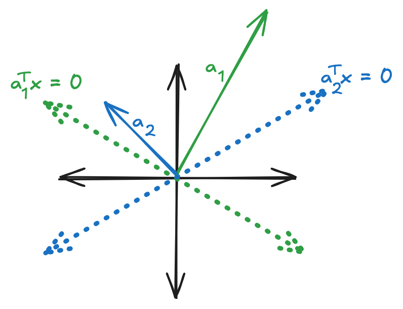
What happens when $b1, b_2 \ne 0$, meaning there is some translation
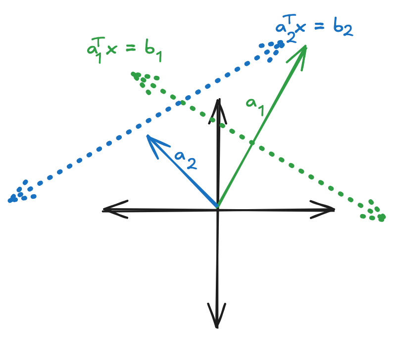
We notice that, since they are lines extending infinitely in both directions, there will always be a point where they intersect.
This leads to the definition of parallel lines - they never intersect. For disjoint sets, we are looking for parallel lines. That means that the lines have to have originated in the same place but translated by different amounts which was what we proved analytically.
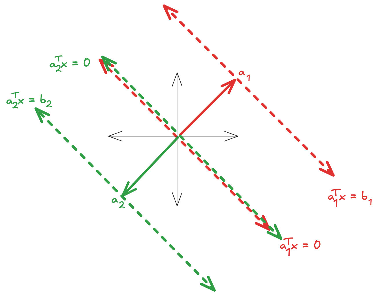
The linear functional view
Another way to view this is from the POV of linear functionals. We can think of each linear functional $a$ as a ruler that tells us how “long” it is in the direction of $a$. The above scenario happens when we ask that the length of some vector $x$ is two different values in the same direction.
b) When $S_1$ and $S_2$ do intersect, what kind of space is $S_1 \cap S_2$? What is its dimension? Please list all the possible cases
Let us first tackle the question about dimensions.
Let us remind ourselves what hyperspaces are. For a vector space $V\subseteq \R^n$ , it’s hyperplane is a flat of dimension $n-1$.
Examples
- For $R^2$ the hyperplane is a 1-dimensional line
- For $R^3$ the hyperplane is a 2-d plane and so on
There are two ways in which flats can intersect
- They coincide
- The intersect and form a new flat of dimension $(n-1)-1$
Hence the dimension of $S_1 \cap S_2$ is either $n-1$ when they coincide or $n-2$ if they intersect
Examples
- For $R^1$ line they intersect at a $R^0$ point
- For a $R^2$ plane they intersect at a $R^1$ line
More rigorous proof of a)
More formally, using more advanced linear algebra, we can prove a) as follows
Let $A = \begin{bmatrix}- a_1 -\newline- a_2 -\end{bmatrix}$
$B = \begin{bmatrix}b_1\newline b_2\end{bmatrix}$
We represent our hyperplanes as a system of linear equations
$Ax = B$
We assume that $\text{rank}(A) = 2$, meaning full rank as we covered the other case above.
If $A$ had been a non-singular matrix, our life would have been much simpler. We could have just multiplied both sides by $A^{-1}$ and be done. Since $A$ is a short-fat matrix, we can’t really take an inverse.
But, we can use SVD (try not to mention SVD challenge: impossible) to find the Moore-Penrose inverse of $A$ to solve the above equation.
$A^{\dagger}$ is defined to be $A^T(AA^T)^{-1}$ if $\text{rank}(A) = 2$ instead of $n$
$A = U\Sigma V^T$
$A^T =V \Sigma^T U^T = V\Sigma U^T$ [$\Sigma$ is $\text{diag}$, therefore symmetric]
$AA^T = U\Sigma V^T(U \Sigma V^T)^T$
$AA^T = U\Sigma V^T(V^T)^T\Sigma^T U^T$
$AA^T = U\Sigma V^T V \Sigma^T U^T$ [We know that $V$ is orthonormal]
$AA^T = U\Sigma \Sigma^T U^T$ [Since $\Sigma$ is a $\text{diag}$, $\Sigma\Sigma^T = \Sigma^2$]
$AA^T = U\Sigma^2 U^T$ [We know that $V$ is orthonormal]
Let us find the inverse
$(AA^T)^{-1} = (U\Sigma^2 U^T)^{-1}$
$(AA^T)^{-1} = (U^T)^{-1} (\Sigma^2)^{-1} U^{-1}$ [$U$ is orthogonal]
$(AA^T)^{-1} = U (\Sigma^2)^{-1} U^{T}$ [$U$ is orthogonal]
Multiplying with $A^T$
$A^T =V \Sigma^T U^T = V\Sigma U^T$ [$\Sigma$ is $\text{diag}$, therefore symmetric]
$(AA^T)^{-1} = U \Sigma^{-1} U^{T}$ [$U$ is orthogonal]
$A^T(AA^T)^{-1} = (V\Sigma U^T)(U(\Sigma^2)^{-1}U^{T})$ [$\Sigma^{-1}$ is the $\text{diag}$ with the reciprocals. Same for $(\Sigma^2)^{-1}$]
$A^T(AA^T)^{-1} = V\Sigma^{-1}U^{T}$
Remember our definition of $A = U\Sigma V^T$, then
$(A^T(AA^T)^{-1})A = V\Sigma^{-1}U^{T}U\Sigma V^T$
$(A^T(AA^T)^{-1})A = I$ [$U, V$ are orthogonal and $\Sigma\Sigma^{-1} = I$]
Hence $A^{\dagger}$ is indeed an inverse
We can solve for $x$ as
$x = A^T(AA^T)^{-1}B$
$= \begin{bmatrix}| && | \newline a_1 && a_2 \newline | && | \end{bmatrix}\Biggl( \begin{bmatrix}- a_1 -\newline- a_2 -\end{bmatrix} \begin{bmatrix}| && | \newline a_1 && a_2 \newline | && | \end{bmatrix}\Biggr)^{-1} \begin{bmatrix}b_1\newline b_2\end{bmatrix}$
$\newcommand{\AT}{\begin{bmatrix}| && | \newline a_1 && a_2 \newline | && | \end{bmatrix}}$ $\newcommand{\A}{\begin{bmatrix}| && | \newline a_1 && a_2 \newline | && | \end{bmatrix}}$
$=\AT\begin{bmatrix}||a_1||^2 && \langle a_1, a_2\rangle \newline \langle a_1, a_2\rangle && ||a_2||^2\end{bmatrix}^{-1}\begin{bmatrix}b_1 \newline b_2\end{bmatrix}$
Inverse of a $2\times2$ is simple enough to calculate by hand,
$=\AT \frac{1}{||a_1||^2||a_2||^2-\langle a_1, a_2\rangle}\begin{bmatrix}||a_2||^2 && -\langle a_1, a_2\rangle \newline -\langle a_1, a_2 \rangle && ||a_1||^2 \end{bmatrix}\begin{bmatrix}b_1 \newline b_2\end{bmatrix}$
$x = \frac{||a_2||^2b_1 - \langle a_1, a_2 \rangle b_2}{||a_1||^2||a_2||^2 - \langle a_1, a_2 \rangle^2} a_1 + \frac{||a_1||^2b_2 - \langle a_1, a_2\rangle b_1}{||a_1||^2||a_2||^2 - \langle a_1, a_2 \rangle^2} a_2$
If we converted $a_1$ and $a_2$ to be unit vectors, let $\tilde{b_1}$ and $\tilde{b_2}$ be the new RHS
Then we have, $||\hat{a_1}|| = ||\hat{a_2}|| = 1$
$\langle \hat{a_1}, \hat{a_2} \rangle = \cos\theta$
$1 - \langle \hat{a_1}, \hat{a_2} \rangle^2 = \sin^2\theta$
Hence,
$\boxed{x = \frac{\tilde{b_1} - \tilde{b_2}\cos\theta}{\sin^2\theta} \hat{a_1} +\frac{\tilde{b_2} - \tilde{b_1}\cos\theta}{\sin^2\theta}\hat{a_2}}$
References
- Strang, Gilbert 29. Singular Value Decomposition [Video]. YouTube. https://www.youtube.com/watch?v=TX_vooSnhm8
- Strang, Gilbert. (2019). Linear Algebra and Learning from Data. Wellesley-Cambridge Press.
- Burton, Steve Linear Systems of Equations, Least Squares Regression, Pseudoinverse [Video] https://youtu.be/PjeOmOz9jSY?si=tqNtcV2RDvXJ6n6C
- Brunton, S. L., & Kutz, J. N. (2019). Data-Driven Science and Engineering: Machine Learning, Dynamical Systems, and Control. Cambridge University Press.
- Rodrigo de Azevedo (https://math.stackexchange.com/users/339790/rodrigo-de-azevedo), How to find the intersection of two hyperplanes in $n$ dimensions?, URL (version: 2017-07-23): https://math.stackexchange.com/q/2369012
4) Convex Cones from Convex Sets
Let $S \subset \R^n$ be a convex set. Define the set
$$ C = \{\theta x: x\in S, \theta \ge 0\} $$
Show that C is a convex cone.
$C$ is a convex cone if $\forall x_1, x_2 \in C$
$\theta_1 x_1 + \theta_2 x_2 \in C, \theta_i \ge 0$
Meaning, pick any two point in the convex cone, the pie in between them is also in the convex cone
Let us establish some notation
Vectors from the cone will be denoted by $x_i$ and vectors from the original convex set will be denoted by $\tilde{x}_i$
$\exists\theta_1, x_1, \theta_2, x_2\text{ s.t. } = \theta_1 x_1 + \theta_2 x_2, \forall x_3 \in C$
We also know that $\exists \tilde{x} \in S, \theta\tilde{x} = x, \forall x\in C$
$x_3 = \theta_1 x_1 + \theta_2 x_2$
$$\lambda_3 \tilde{x}_3 = \theta_1 \lambda_1\tilde{x}_1 + \theta_2\lambda_2 \tilde{x}_2\tag{1}$$
Since $\tilde{x}_1, \tilde{x}_2 \in S$, w.k.t
$\tilde{x}_1 + \varphi (\tilde{x}_1 - \tilde{x}_2)\in S, \forall \varphi \in [0, 1]$
This means that
$\theta (\tilde{x}_1 + \varphi (\tilde{x}_1 - \tilde{x}_2)) \in C, \forall \theta \ge0$
Consider the RHS of (1)
Let us multiply and divide by $\frac{\theta_1\lambda_1 + \theta_2\lambda_2}{\theta_1\lambda_1 + \theta_2\lambda_2}$
(Without rigorous proof assume that all the terms are never equal to 0 simultaneously. If they were then we would only have $\{0\}$, which is easily provable to be a convex cone)
$\frac{\theta_1\lambda_1 + \theta_2\lambda_2}{\theta_1\lambda_1 + \theta_2\lambda_2} (\theta_1\lambda_1\tilde{x}_1 + \theta_2\lambda_2\tilde{x}_2)$
$= (\theta_1\lambda_1 + \theta_2\lambda_2)(\frac{\theta_1\lambda_1}{\theta_1\lambda_1 + \theta_2\lambda_2}\tilde{x}_1 +\frac{\theta_2\lambda_2}{\theta_1\lambda_1 + \theta_2\lambda_2}\tilde{x}_2 )$
Notice that
$\frac{\theta_1\lambda_1}{\theta_1\lambda_1 + \theta_2\lambda_2} + \frac{\theta_2\lambda_2}{\theta_1\lambda_1 + \theta_2\lambda_2} = 1$
We can rewrite $\frac{\theta_2\lambda_2}{\theta_1\lambda_1 + \theta_2\lambda_2} = 1 -\frac{\theta_1\lambda_1}{\theta_1\lambda_1 + \theta_2\lambda_2}$
We get
$= (\theta_1\lambda_1 + \theta_2\lambda_2)(\frac{\theta_1\lambda_1}{\theta_1\lambda_1 + \theta_2\lambda_2}\tilde{x}_1 + (1 -\frac{\theta_1\lambda_1}{\theta_1\lambda_1 + \theta_2\lambda_2}) \tilde{x}_2 )$
Since $\tilde{x}_1, \tilde{x}_2 \in S$ w.k.t
$\theta \tilde{x}_1 + (1-\theta)\tilde{x}_2 \in S$
Here $\theta =\frac{\theta_1\lambda_1}{\theta_1\lambda_1 + \theta_2\lambda_2}$
Let us call this $\tilde{x}^*$
$=(\theta_1\lambda_1 + \theta_2\lambda_2)\tilde{x}^*$
$\theta_1, \theta_2, \lambda_1, \lambda_2 \ge0 \implies \theta_1\lambda_1 + \theta_2\lambda_2 \ge 0$
$= \theta \tilde{x}^*$
Which is in $C$ by definition. Hence proved $\hp$
5) Convex Combinations and Convex Functions
a) Let $C \subset \R^n$ be a convex set, and let $f: C \rightarrow \R$ be a convex function. Show that for any $x_1, \ldots, x_n \in C$ and any $\theta_1\ldots,\theta_k \ge0$, with $\sum \theta_i = 1$
$$ f(\theta_1x_1 + \ldots + \theta_k x_k) \le \theta_1 f(x_1) + \ldots \theta_k f(x_k)$$
We notice that this is Jensen’s inequality.
By the definition of convex functions, we already know that
$$f(\theta x + (1 - \theta) y) \le \theta f(x) + (1 - \theta) f(y), \theta \in [0, 1]$$
The above inequality extends it to any convex combination of a subset of $C$
This setup of this problem is strikingly similar to the proof we did for affine sets. Let us prove this using induction
Base case
The base case of $k = 2$ is proven axiomatically through the definition of convexity.
Induction step
Let us assume that for some $k-1$ it is true that
$$ f(\theta_1x_1 + \ldots + \theta_{k-1} x_{k-1}) \le \theta_1 f(x_1) + \ldots +\theta_{k-1} f(x_{k-1}), \sum_{i=1}^{k-1} \theta_i = 1$$
We want to show that
$$ f(\theta_1x_1 + \ldots + \theta_k x_k) \le \theta_1 f(x_1) + \ldots \theta_k f(x_k), \sum_{i=1}^{k}\theta_i = 1$$
I want to clarify that the $\theta$s are merely to represent the weights and are not the same constants i.e for any set of $k-1$ weights $\theta$s summing up to 1, our assumption holds.
We know that our weights have to sum up to one
$\sum_{i = 1}^{k} \theta_i = 1$
$\theta_1 +\theta_2+\ldots+\theta_{k-1} + \theta_k = 1$ $\theta_1 +\theta_2+\ldots+\theta_{k-1} = 1- \theta_k$
Assuming $\theta_k \ne 1$ (which is a safe assumption as that branch of the proof is merely $f(x_k) = f(x_k)$), we can divide by $1-\theta_k$ to get
$\frac{\theta_1}{1 - \theta_k} + \ldots \frac{\theta_{k-1}}{1 - \theta_k} = 1$
Notice that we have $k-1$ weights summing up to 1. That means
$\implies f(\frac{\theta_1}{1 - \theta_k} x_1 + \ldots \frac{\theta_{k-1}}{1 - \theta_k} x_{k-1}) \le \frac{\theta_1}{1 - \theta_k} f(x_1) + \ldots + \frac{\theta_{k-1}}{1 - \theta_k} f(x_{k-1})$
Since $C$ is a convex set, any convex combinations of its points will also be in the set
Let us call this $\frac{\theta_1}{1 - \theta_k} x_1 + \ldots \frac{\theta_{k-1}}{1 - \theta_k} x_{k-1}$ as $\tilde{x}$
$$f(\tilde{x}) \le \frac{\theta_1}{1 - \theta_k} f(x_1) + \ldots + \frac{\theta_{k-1}}{1 - \theta_k} f(x_{k-1})\tag{1}$$
Using the definition of a convex function, we can say that
$f((1-\theta_k)\tilde{x} + \theta_k x_k) \le (1-\theta_k)f(\tilde{x}) + \theta_k f(x_k)$
We know the upper bound of $f(\tilde{x})$ from $(1)$
$f((1-\theta_k)\tilde{x} + \theta_k x_k) \le (1-\theta_k) (\frac{\theta_1}{1 - \theta_k} f(x_1) + \ldots + \frac{\theta_{k-1}}{1 - \theta_k} f(x_{k-1}))+ \theta_k f(x_k)$
$f((1-\theta_k)\tilde{x} + \theta_k x_k) \le {\theta_1} f(x_1) + \ldots + \theta_{k-1} f(x_{k-1})+ \theta_k f(x_k)$
Expanding $\tilde{x}$
$f(\theta_1x_1 + \ldots + \theta_k x_k) \le \theta_1 f(x_1) + \ldots \theta_k f(x_k)\hp$
b) Let $f: \R^n \rightarrow \R$ be a convex function. Show that for any $x_1, \ldots, x_k \in \R^n$ and any $\theta_1 \ge 0, \theta_{i\in[2, k]}\le 0$ with $\sum\theta_i = 1$
$$f(\theta_1x_1 + \ldots + \theta_k x_k) \ge \theta_1f(x_1) + \ldots + \theta_k f(x_k)$$
Here we are asked if the graph of the left side of an affine combination is greater than the affine combination itself.
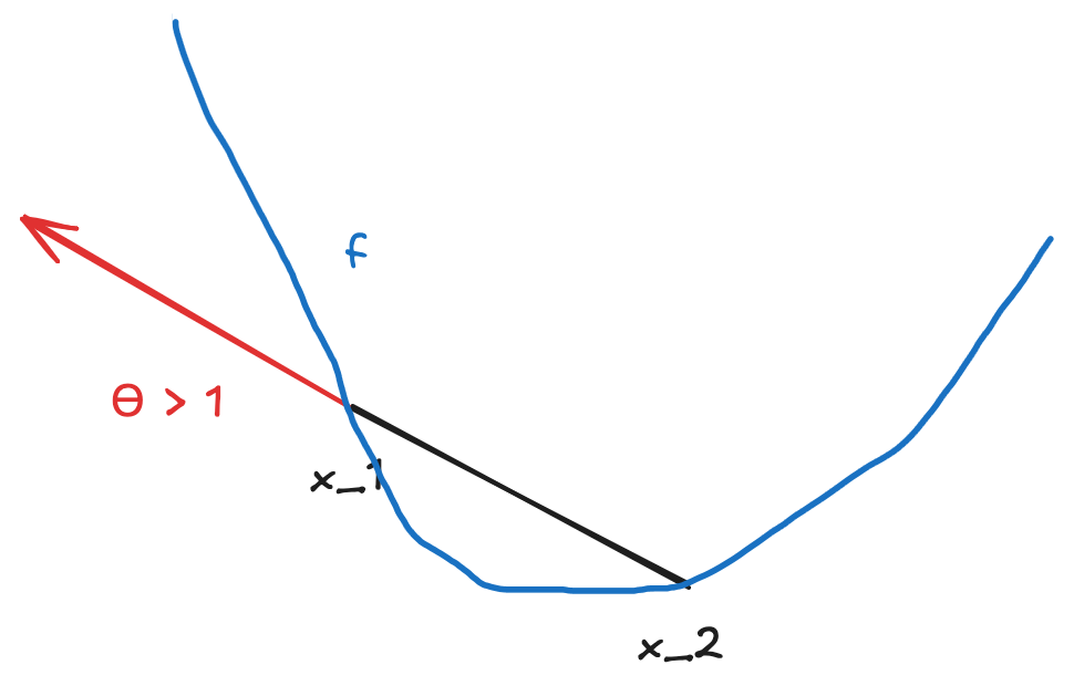
Similar to last problem, let us solve it by induction
Base case $n = 2$
$f(\theta_1 x_1 + \theta_2 x_2) \ge \theta_1 f(x_1) + \theta_2 f(x_2)$
We know that $\theta_1 + \theta_2 = 1$
Lets just have one $\theta$
$f(\theta x_1 + (1-\theta) x_2) \ge \theta f(x_1) + (1-\theta) f(x_2)$
We know that this is a line passing through $x_1$ and $x_2$
Let us pick a arbitrary point with some $\theta$ and $x_2$
Since $f$ is convex,
We can say that $f(\lambda(\theta x_1 + (1-\theta) x_2) + (1 - \lambda) x_2) \le \lambda f(\theta x_1 + (1-\theta) x_2) + (1-\lambda)f(x_2)$
This is the line between $x_2$ and some point $\theta x_1 + (1-\theta) x_2$
We know that $x_1$ lies on this line and $\lambda = \frac{1}{\theta}$
Substituting we find,
$f(\frac{1}{\theta}(\theta x_1 + (1-\theta) x_2) + (1 - \frac{1}{\theta}) x_2) \le \frac{1}{\theta} f(\theta x_1 + (1-\theta) x_2) + (1-\frac{1}{\theta})f(x_2)$
$f(x_1) \le \frac{1}{\theta}f(\theta x_1 + (1 - \theta)x_2) + (1-\frac{1}{\theta})f(x_2)$
$f(x_1) \le \frac{1}{\theta}[f(\theta x_1 + (1-\theta)x_2) - (1-\theta)f(x_2)]$
$\theta f(x_1) + (1-\theta)f(x_2) \le f(\theta x_1 + (1-\theta)x_2)$
$f(\theta x_1 + (1-\theta)x_2) \ge \theta f(x_1) + (1-\theta)f(x_2)$
Induction
Let us assume for some $k$, $k-1$ is true
$f(\theta_1 x_1 + \ldots + \theta_{k-1} x_{k-1}) \ge \theta_1 f(x_1) +\ldots + \theta_{k-1}f(x_{k-1})$
if $\sum_{i = 1}^{k-1} \theta_i = 1, \theta_1 \gt 0, \theta_{i\in[2, k-1]} \le 0$
That is if we have $k-1$ weights summing up to 1 with the first one being the only one positive and all the other non-positive, we have the above inequality
We have to prove that
$$f(\theta_1x_1 + \ldots + \theta_k x_k) \ge \theta_1f(x_1) + \ldots + \theta_k f(x_k)$$
We know that
$\theta_1 + \theta_2 + \ldots + \theta_k = 1$
$\theta_1 + \theta_2 + \ldots + \theta_{k-1} = 1$
The induction goes the same as above. $\tilde{x}$ will take the place of $x_2$. We are adding $x_1$ to $\tilde{x}$ instead of $x_2$
References
- I discussed 5b) with Logan Foster (
zup7mn)
6) Convex function or not?
- c) $\log\frac{\exp(a^Tx +b)}{1 + \exp(a^Tx+b)}$ for $a\in \R^n\setminus\{0\}, b\in\R$
$\log(\exp(a^Tx+b)) - \log(\frac{1}{1+\exp(a^Tx+b)})$
$a^Tx+b - \log(\frac{1}{1+\exp(a^Tx+b)})$
$\exp$ is convex for any $\R$, hence $\exp(a^Tx +b)$ is convex
$\frac{1}{1 + e^x} \in \R_{++}$
Hence the $\log$ becomes concave, which means $-\log$ is convex
We have an affine transformation plus a convex function which is convex
7)
- When is the epigraph of a function a halfspace?
- When the epigraph of a function is a half space, it means that the graph divides the spaces into two convex set. Which would mean that the epigraph is a convex set. If the epigraph is a convex set then $f$ must be a convex function.
- If the epigraph is a half-space then the hypograph is also an halfspace. Which means that the function is also concave
- Hence the function must be affine.